The TL;DR
The core commandments of personal finance are almost embarrassingly simple:
- Increase your earning power (expand the top of the funnel).
- Spend less than you earn (live below your means).
- Invest the difference as soon as you have it (deploy money the moment you have it to invest; never hoard cash on the sidelines trying to time the market).
- Diversify ruthlessly (the only free lunch in finance; tame volatility drag).
- Stay liquid (maintain an emergency buffer so market dips never force you to sell).
- Seek asymmetric bets (cap your downside, but leave room for explosive positive jumps).
- Wait (give compound interest the runway to work its exponential magic).
That’s the core canon—seven principles that cover nearly everything you need to know. Everything else is mostly commentary.
Yet human beings instinctively treat simple advice with suspicion. When the formula for building wealth boils down to living below your means, investing surplus cash, and waiting, it feels too basic to be trusted. We convince ourselves there must be a catch, a cheat code, or some hidden secret sauce that sophisticated insiders keep to themselves.
The Rule of 72 is often where that search begins. It looks like a clever arithmetic hack—a mental math trick promising a shortcut to understanding how fast money grows.
Here is the spoiler up front: for all practical purposes, the Rule of 72 is completely useless.
It isn’t useless because the basic math is wrong; but because real markets violently violate every single assumption the formula takes for granted. In this essay, we will take the exact mathematical foundation the Rule of 72 is built upon, follow that same math to its logical conclusion in the real world, and prove why planning your financial life around a deterministic doubling target is an illusion.
We’re going to take the deceptively innocent question—“How long will it take for my money to double?”—and climb the escalation ladder:
- Level 1: The Cocktail Party Rule ($t \approx 72/r$)
- Level 2: Peeling the Onion (Logarithms, Taylor series, and why 72 beats 69.3)
- Level 3: The Ghost in the Ledger (Inflation and the brutal erosion of purchasing power)
- Level 4: The Volatility Drag (Why a $+50\%$ and $-50\%$ return leaves you broke)
- Level 5: Entering the Stochastic Matrix (Geometric Brownian Motion and First Passage Time)
- Level 6: Shattering the Assumptions (Stochastic Volatility, Regime Shifts, and Market Jumps)
- Level 7: Practical Epiphanies (Why you’re asking the wrong question)
As you’ll see, the journey doesn’t uncover a secret backdoor or an investing shortcut. It leads straight into volatility drag, fat tails, and ruin boundaries—demonstrating that all the relevant rules were already sitting on the table, and that chasing the “secret sauce” leads nowhere nice.
Level 1: The Cocktail Party Rule ($t \approx 72/r$)
Every now and then, someone at a dinner party or on YouTube / TikTok drops a classic mental math trick: The Rule of 72.
It’s an empirical shortcut to estimate how many years it takes for an investment to double at a constant annual compound rate:
$$t \approx \frac{72}{r}$$where:
- $t$ is the time in years to double your capital.
- $r$ is the annual compound interest rate expressed as a percentage (e.g., for an $8\%$ return, $r = 8$, not $0.08$).
Why does everyone love the number 72? Because 72 is an arithmetic masterpiece. It is abundantly composite: it divides cleanly by $2, 3, 4, 6, 8, 9, 12, 18, 24,$ and $36$. You can calculate doubling times in your head between sips of your drink:
- At $4\%$: $\frac{72}{4} = 18$ years
- At $6\%$: $\frac{72}{6} = 12$ years
- At $8\%$: $\frac{72}{8} = 9$ years
- At $10\%$: $\frac{72}{10} = 7.2$ years
- At $12\%$: $\frac{72}{12} = 6$ years
It’s neat, fast, and memorable. But where on earth does the number 72 actually come from? Why not 70? Or 100?
Level 2: Peeling the Onion — Where Does 72 Actually Come From?
Suppose you start with an initial principal $P_0$. If it compounds annually at a fractional rate $R = r / 100$, your wealth after $t$ years is:
$$P(t) = P_0 (1 + R)^t$$To double your money, we want $P(t) = 2 P_0$. Substituting:
$$P_0 (1 + R)^t = 2 P_0 \implies (1 + R)^t = 2$$Notice the initial amount $P_0$ cancels out immediately. Whether you’re trying to turn $100 into $200 or $10,000,000 into $20,000,000, the doubling time is identical.
Now, take the natural logarithm ($\ln$) of both sides:
$$\ln\left((1 + R)^t\right) = \ln(2)$$$$t \ln(1 + R) = \ln(2)$$Solving for $t$:
$$t = \frac{\ln(2)}{\ln(1 + R)}$$We know that $\ln(2) \approx 0.693147$. So the exact doubling time is:
$$t = \frac{0.693147}{\ln(1 + R)}$$The First-Order Taylor Approximation
Evaluating $\ln(1 + R)$ in your head is not recommended at social gatherings. Fortunately, calculus gives us the Taylor series expansion of $\ln(1 + x)$ around $x = 0$:
$$\ln(1 + x) = x - \frac{x^2}{2} + \frac{x^3}{3} - \frac{x^4}{4} + \cdots$$For small interest rates ($R \ll 1$), the higher-order terms ($x^2, x^3, \dots$) are tiny. Truncating at the first term yields the linear approximation:
$$\ln(1 + R) \approx R$$Substitute this back into our formula:
$$t \approx \frac{0.693147}{R}$$Converting $R$ back to a percentage $r$ ($r = 100 R$):
$$t \approx \frac{69.3147}{r}$$Technically speaking, if interest compounded continuously (where $P(t) = P_0 e^{Rt}$), the exact doubling time would be identically $t = \frac{\ln(2)}{R} = \frac{69.3}{r}$.
So why does the popular rule use 72 instead of 69.3?
The Two Reasons 72 Wins
- Divisibility: As noted earlier, dividing 69.3 by 7 or 8 in your head is an exercise in misery. 72 is far kinder to the human brain.
- The Higher-Order Correction: For discrete annual compounding, the linear approximation $\ln(1 + R) \approx R$ slightly overestimates $\ln(1 + R)$.
If we include the second-order term of the Taylor series:
$$\ln(1 + R) \approx R\left(1 - \frac{R}{2}\right)$$Plugging this into the denominator:
$$t \approx \frac{\ln(2)}{R\left(1 - \frac{R}{2}\right)} \approx \frac{\ln(2)}{R} \left(1 + \frac{R}{2}\right)$$Since $\ln(2) \approx 0.693$:
$$t \approx \frac{69.3}{r} + \frac{0.693 \times 100 \times R}{2 \times 100 R} \approx \frac{69.3}{r} + 0.35$$Alternatively, we can express the numerator itself as an adjusted constant $N(r) \approx 69.3 \times (1 + R/2)$. For typical annual market returns between $6\%$ and $10\%$ ($R = 0.06$ to $0.10$):
$$N(8\%) \approx 69.3 \times \left(1 + \frac{0.08}{2}\right) = 69.3 \times 1.04 \approx 72.07$$Notice how close that gets. At an $8\%$ return:
- Exact formula: $t = \frac{\ln(2)}{\ln(1.08)} = 9.0065$ years.
- Rule of 72: $t = \frac{72}{8} = 9.0000$ years.
The error is less than $0.07\%$! The shift from 69.3 to 72 isn’t just a convenience for mental arithmetic; it actually compensates for the curvature of discrete annual compounding.
| Rate ($r$) | Exact $t = \frac{\ln(2)}{\ln(1+R)}$ | Rule of 72 ($72/r$) | Rule of 69.3 ($69.3/r$) | Error (72 vs Exact) |
|---|---|---|---|---|
| 2% | 35.00 yrs | 36.00 yrs | 34.65 yrs | $+2.8\%$ |
| 4% | 17.67 yrs | 18.00 yrs | 17.33 yrs | $+1.8\%$ |
| 6% | 11.90 yrs | 12.00 yrs | 11.55 yrs | $+0.8\%$ |
| 8% | 9.01 yrs | 9.00 yrs | 8.66 yrs | $-0.07\%$ |
| 10% | 7.27 yrs | 7.20 yrs | 6.93 yrs | $-1.0\%$ |
| 12% | 6.12 yrs | 6.00 yrs | 5.78 yrs | $-1.9\%$ |
Level 3: The Ghost in the Ledger — Inflation & Real Purchasing Power
There is, however, an immediate complication.
Suppose your investment account doubles from $100,000 to $200,000. That looks great on a statement. But if everyday goods and services have also doubled in cost over that period, you haven’t actually built wealth—you’ve merely kept pace with an eroding unit of account.
Nominal doubling is an accounting milestone, but what you actually care about is real purchasing power doubling.
Let $\pi$ be the annual inflation rate (as a fraction, so $i = 100\pi$ is the percentage). After $t$ years, the price level has multiplied by $(1 + \pi)^t$. Therefore, your real wealth $V(t)$ measured in base-year purchasing power is:
$$V(t) = \frac{P(t)}{(1 + \pi)^t} = P_0 \left( \frac{1 + R}{1 + \pi} \right)^t$$For your real purchasing power to double ($V(t) = 2 P_0$):
$$\left( \frac{1 + R}{1 + \pi} \right)^t = 2$$Taking logarithms:
$$t \cdot \left[ \ln(1 + R) - \ln(1 + \pi) \right] = \ln(2)$$$$t_{\text{real}} = \frac{\ln(2)}{\ln(1 + R) - \ln(1 + \pi)}$$The Real Rule of 72
Using our Taylor expansion $\ln(1 + x) \approx x$:
$$\ln(1 + R) - \ln(1 + \pi) \approx R - \pi$$So the real doubling time becomes:
$$t_{\text{real}} \approx \frac{72}{r - i}$$where $r - i$ is the real rate of return (the classic Fisher relation approximation).
The Sobering Reality Check
Let’s see what happens to an investor earning an apparently healthy $8\%$ nominal return:
| Inflation Rate ($i$) | Real Return ($r - i$) | Exact Real Doubling Time | What Happened? |
|---|---|---|---|
| $0\%$ | $8.0\%$ | 9.0 years | Paradise |
| $2\%$ | $5.9\%$ | 12.1 years | Central bank target (+3 yrs delay) |
| $3\%$ | $4.9\%$ | 14.6 years | Historical US baseline (+5.6 yrs delay) |
| $5\%$ | $2.9\%$ | 24.5 years | Moderate inflation (+15.5 yrs delay!) |
| $7\%$ | $0.9\%$ | 74.8 years | You’ll double in retirement… maybe |
Notice the non-linearity. A jump from $2\%$ to $5\%$ inflation doesn’t just slow down your doubling time by a modest increment—it doubles the time needed to double your real wealth, from $12$ years to nearly $25$ years.
Inflation is an exponential headwind masquerading as a linear annoyance.
Level 4: The Illusion of Constant Returns — Volatility Drag
So far, we have made a polite and wildly unrealistic assumption: that your return $R$ is identical year after year.
In the real world, asset returns fluctuate. And when returns fluctuate, a nasty mathematical phenomenon emerges: volatility drag (sometimes called variance drain).
The Painful Arithmetic Trap
Consider a simple two-year bet:
- Year 1: Your portfolio gains $+50\%$.
- Year 2: Your portfolio drops $-50\%$.
What was your average annual return?
$$\bar{R}_{\text{arithmetic}} = \frac{+50\% + (-50\%)}{2} = 0\%$$On paper, your arithmetic average is zero. You might think you broke even. Let’s check your actual balance:
- Start with $100.
- After Year 1 ($+50\%$): $100 $\times 1.50 =$ $150.
- After Year 2 ($-50\%$): $150 $\times 0.50 =$ $75.
You didn’t break even. You lost $25\%$ of your money.
Why? Because compounding depends on the geometric mean, not the arithmetic mean. And by the Arithmetic Mean–Geometric Mean (AM-GM) inequality:
$$\text{Geometric Mean} \le \text{Arithmetic Mean}$$The equality holds if and only if all returns are strictly identical. The moment volatility enters the picture, your geometric growth rate falls below your arithmetic average.
Quantifying the Drag
If annual returns have an arithmetic mean $\mu$ and annual variance $\sigma^2$, the long-run compound growth rate $g$ is approximated by:
$$g \approx \mu - \frac{\sigma^2}{2}$$This formula comes directly from a second-order Taylor expansion of expected log-returns (or Itô’s Lemma, which we will see in a moment).
Look closely at that penalty term: $\frac{\sigma^2}{2}$.
If an asset has an arithmetic average return of $\mu = 10\%$ ($0.10$), but high annual volatility of $\sigma = 20\%$ ($0.20$):
$$g \approx 0.10 - \frac{0.20^2}{2} = 0.10 - \frac{0.04}{2} = 0.10 - 0.02 = 8\%$$Your effective doubling rate isn’t $10\%$; it’s $8\%$. That drops your doubling speed from $7.2$ years to $9.0$ years.
What if you invest in an ultra-volatile tech stock or crypto token with $\mu = 20\%$ but $\sigma = 60\%$?
$$g \approx 0.20 - \frac{0.60^2}{2} = 0.20 - \frac{0.36}{2} = 0.20 - 0.18 = 2\%$$The arithmetic average says $20\%$, but your actual compound growth rate is a pitiful $2\%$. At that rate, doubling takes $\frac{72}{2} = 36$ years! Volatility didn’t just add excitement; it vaporized your compounding engine.
Level 5: Entering the Stochastic Matrix — First Passage Time
Up to this point, we have treated doubling time as a deterministic number. But in reality, the time it takes to double your money is not a constant $t$—it is a random variable $T$ with its own probability distribution.
Let’s formalize this using continuous-time finance.
Modeling Wealth as Geometric Brownian Motion
Model the price of an investment asset $S_t$ using the standard Geometric Brownian Motion (GBM):
$$dS_t = \mu S_t dt + \sigma S_t dW_t$$where:
- $\mu$ is the expected arithmetic drift rate.
- $\sigma$ is the volatility.
- $W_t$ is a standard Wiener process (Brownian motion), where increments $dW_t \sim \mathcal{N}(0, dt)$.
To solve this stochastic differential equation, we apply Itô’s Lemma to the function $f(S_t) = \ln(S_t)$:
$$d(\ln S_t) = f'(S_t) dS_t + \frac{1}{2} f''(S_t) (dS_t)^2$$Since $f'(S) = \frac{1}{S}$ and $f''(S) = -\frac{1}{S^2}$, and using $(dS_t)^2 = \sigma^2 S_t^2 dt$:
$$d(\ln S_t) = \frac{1}{S_t}(\mu S_t dt + \sigma S_t dW_t) - \frac{1}{2}\frac{1}{S_t^2}(\sigma^2 S_t^2 dt)$$$$d(\ln S_t) = \left( \mu - \frac{1}{2}\sigma^2 \right) dt + \sigma dW_t$$Integrating from time $0$ to $t$:
$$\ln\left(\frac{S_t}{S_0}\right) = \left( \mu - \frac{1}{2}\sigma^2 \right) t + \sigma W_t$$Notice the effective drift term: $\alpha = \mu - \frac{1}{2}\sigma^2$. The volatility drag penalty appears here not as an empirical rule of thumb, but directly from the second derivative of the logarithm in Itô’s calculus.
The Doubling Problem as an Absorbing Barrier
Doubling your money means reaching the wealth level $S_t = 2 S_0$, which is equivalent to:
$$\ln\left(\frac{S_t}{S_0}\right) = \ln(2)$$Define the doubling time $T$ as the first time the process reaches the threshold $\ln(2)$:
$$T = \inf \left\{ t > 0 : \alpha t + \sigma W_t \ge \ln(2) \right\}$$where $\alpha = \mu - \frac{1}{2}\sigma^2$.
In probability theory, this is the classic First Passage Time of a Brownian motion with drift to an absorbing barrier.
The Inverse Gaussian (Wald) Distribution
Assuming positive net drift $\alpha > 0$, the random variable $T$ follows an Inverse Gaussian (Wald) distribution $\mathcal{IG}$:
$$T \sim \text{InverseGaussian}\left(\mu_T, \lambda\right)$$with parameters:
- Mean: $\mu_T = \frac{\ln(2)}{\alpha} = \frac{\ln(2)}{\mu - \frac{1}{2}\sigma^2}$
- Shape parameter: $\lambda = \frac{(\ln(2))^2}{\sigma^2}$
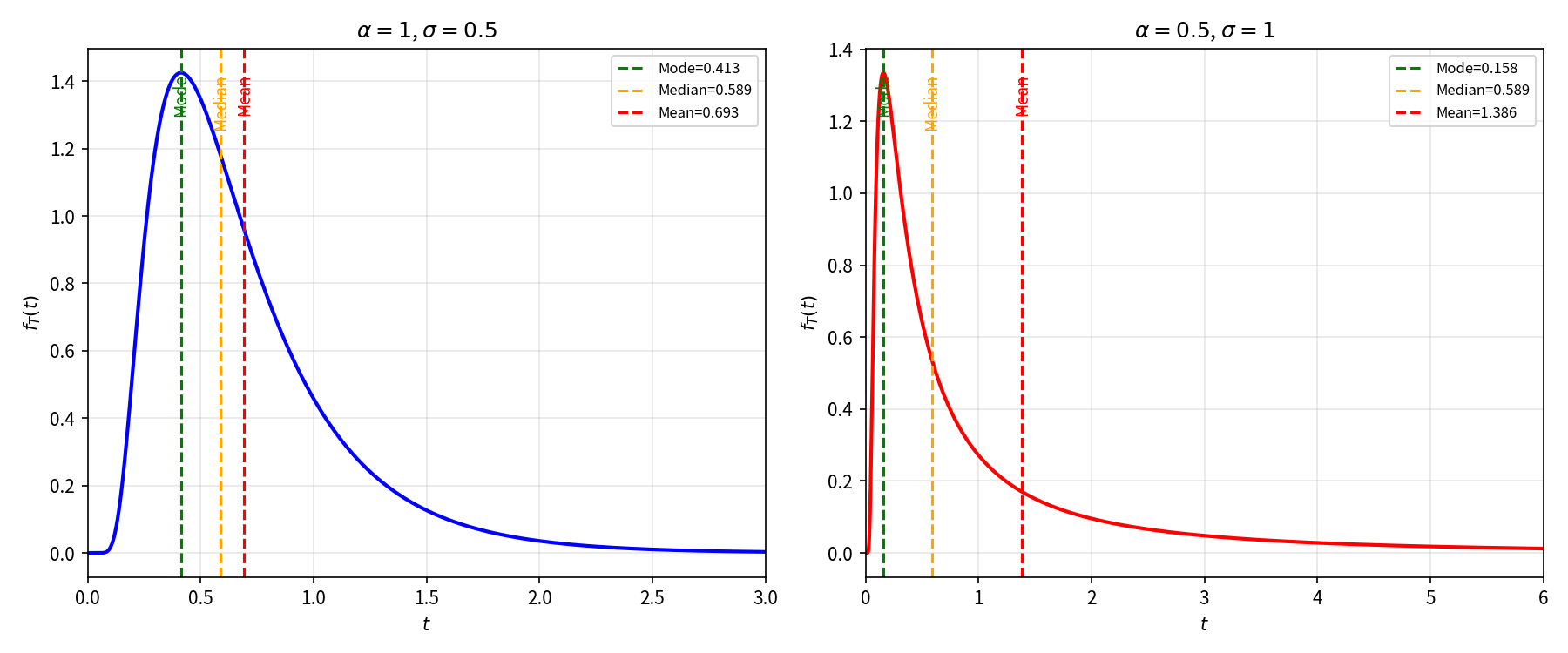
The probability density function (PDF) of the doubling time $t$ is given by:
$$f_T(t) = \frac{\ln(2)}{\sqrt{2\pi \sigma^2 t^3}} \exp\left( -\frac{(\ln(2) - \alpha t)^2}{2\sigma^2 t} \right), \quad t > 0$$Several important properties follow from this distribution:
-
Severe Positive Skew: The distribution of doubling times is not a symmetric bell curve. It has a steep left wall (it is physically hard for a continuous process with modest volatility to double overnight) and a long, fat right tail.
-
Mode < Median < Mean:
- The mode (the single most likely year you double) is earlier than the median.
- The median time to double is $t_{\text{median}} \approx \frac{\ln(2)}{\alpha}$. Half of the possible universes double before this date, half take longer.
- The mean (expected value) is pulled far to the right by the unlucky timelines where markets endure protracted bear cycles.
-
The Probability of Never Doubling: What if your portfolio’s drift is negative ($\alpha \le 0$)? For example, what if you hold an asset where inflation and volatility drag exceed your expected return?
The probability that you ever double your money is:
$$\mathbb{P}(T < \infty) = \begin{cases} 1 & \text{if } \alpha \ge 0 \\ \exp\left( \frac{2\alpha \ln(2)}{\sigma^2} \right) < 1 & \text{if } \alpha < 0 \end{cases}$$If net drift is negative, there is a strictly non-zero probability that you will literally die of old age before your portfolio reaches $2 \times P_0$.
Level 6: Shattering the Assumptions
The Inverse Gaussian distribution gives an elegant closed-form result for doubling time under Geometric Brownian Motion.
In practice, however, standard GBM rests on three assumptions that real financial markets routinely violate:
- Volatility $\sigma$ is constant.
- Drift $\mu$ is constant.
- Price paths are continuous (no sudden gaps or jumps).
Here is what happens when those assumptions break down.
1. Volatility Has Its Own Volatility (Stochastic Volatility)
In reality, volatility is not a fixed parameter carved into stone tablets. It clusters (calm months are followed by calm months; turbulent days breed turbulent days) and exhibits an asymmetric leverage effect - when stock prices plunge, market panic causes volatility to violently spike.
Instead of constant $\sigma$, quantitative finance models variance $v_t = \sigma_t^2$ as its own stochastic process. The gold standard is the Heston Stochastic Volatility Model:
$$dS_t = \mu S_t dt + \sqrt{v_t} S_t dW_t^S$$$$dv_t = \kappa(\theta - v_t)dt + \xi \sqrt{v_t} dW_t^v$$where:
- $\theta$ is the long-term mean variance, and $\kappa$ is the rate of mean reversion.
- $\xi$ is the “volatility of volatility” (how wildly variance swings).
- $W_t^S$ and $W_t^v$ are Brownian motions with negative correlation: $\text{Corr}(dW_t^S, dW_t^v) = \rho < 0$.
What this does to your doubling time: Because $\rho < 0$, a sudden downward price drop triggers an instantaneous surge in variance $v_t$.
Recall our volatility drag formula from Level 4: the growth rate penalty is $\frac{v_t}{2}$. This means precisely when your portfolio is down in a deep hole, the drag penalty expands. Recovering from drawdowns takes longer than pure GBM predicts, stretching the fat right tail of the doubling time distribution even further.
2. Drift is Not Constant — Enter Regime Switching
Assuming a constant drift $\mu = 8\%$ implies economic output compounds at an unvarying pace indefinitely.
In truth, economies cycle through distinct macroeconomic regimes:
- Expansion regimes: High drift, low volatility (e.g., the 1990s tech boom or 2010s bull market).
- Stagflation/Crisis regimes: Zero or negative real drift, high volatility (e.g., the 1970s, or the S&P 500’s “Lost Decade” from 2000 to 2010 where the 10-year annualized return was $-0.95\%$).
We can model this using a Markov-Switching Model (Hamilton, 1989), where drift and volatility are governed by a hidden discrete Markov chain $s_t \in \{1, 2, \dots, K\}$:
$$dS_t = \mu(s_t) S_t dt + \sigma(s_t) S_t dW_t$$with a transition probability matrix $\mathbf{P}$ determining how often the market flips between regimes.
What this means for doubling: Your time to double becomes acutely path-dependent based on the order of states you encounter—a phenomenon financial planners call Sequence of Returns Risk. If you enter the market at the dawn of a 10-year stagnant regime, your expected doubling time isn’t just delayed by 10 years; your early compounding momentum is paralyzed, requiring a massive subsequent bull run just to break even.
3. Markets Don’t Just Walk — They Teleport (Jumps & Discontinuities)
Brownian motion paths are continuous almost surely ($t \mapsto W_t$ is continuous). That means to fall from $100 to $70—or to rise from $100 to $200—the asset price must visit $99, $98, or $150, and every single real number along the path.
Real markets don’t care about continuity. Between overnight geopolitical shocks, earnings surprises, buyout bids, and liquidity vacuums, prices jump.
And jumps aren’t just catastrophic crashes—they cut both ways:
- The Downward Teleports: Black Monday in October 1987 (-22.6% in a single session), the March 2020 COVID circuit breakers, or sudden crypto exchange insolvencies.
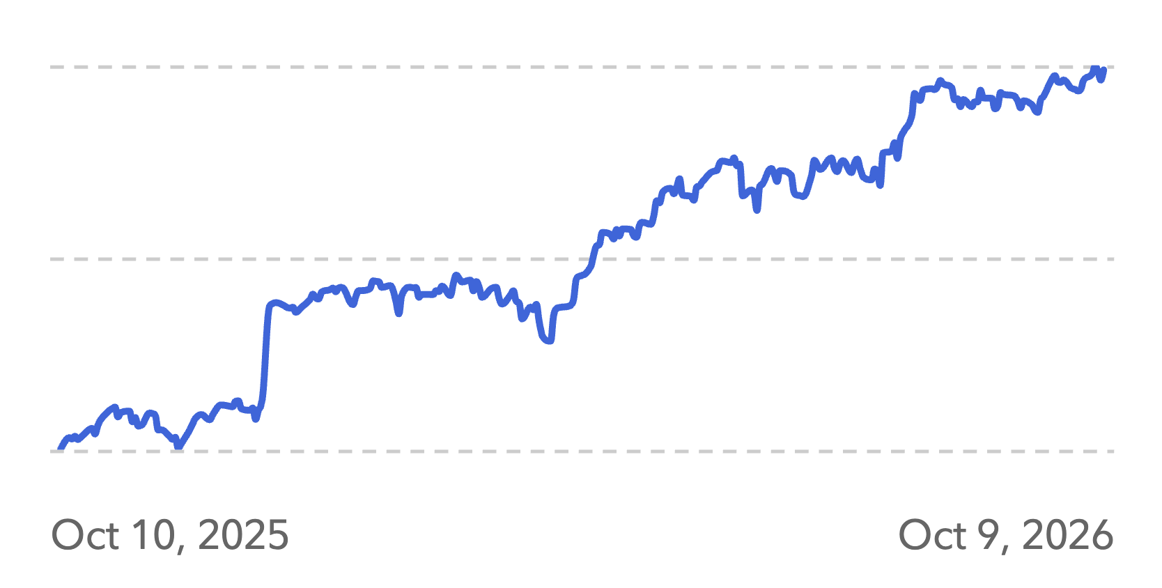
- The Upward Windfalls: Overnight acquisition bids (like SanDisk leaping +28% when Western Digital announced its $19 billion takeover offer, or similar buyout premiums), blockbuster AI guidance (SanDisk shares surging over 575% in 2026, Intel also up over 200% in 2026), binary FDA approvals where clinical-stage biotech stocks gap up +100% to +200% at the opening bell, and violent macro relief rallies (the S&P 500 surging +11.6% on October 13, 2008, or +9.4% on March 24, 2020).
To account for these discontinuous shocks, Robert Merton introduced the Jump-Diffusion Model (Merton, 1976):
$$dS_t = \mu S_t dt + \sigma S_t dW_t + (J_t - 1) S_t dN_t$$where:
- $N_t$ is a Poisson counting process with intensity $\lambda$ (the average frequency of jump events per year).
- $J_t$ is the random jump multiplier. If $J_t = 0.80$, the asset instantly drops by $20\%$ (a crash). If $J_t = 1.30$, it instantly surges by $30\%$ (a windfall). Typically, log-jump sizes follow a normal distribution $\ln(J_t) \sim \mathcal{N}(\mu_J, \sigma_J^2)$, or an asymmetric double-exponential distribution (Kou, 2002) reflecting steep crashes and explosive windfalls.
What jumps do to the doubling barrier:
- Barrier Overshooting & Instant Doubling: In pure GBM, the asset touches the doubling threshold $\ln(2)$ smoothly at an exact instant. In jump-diffusion, an explosive positive jump can launch the asset past the threshold instantaneously. If a buyout offer or breakthrough clinical trial arrives with $J_t \ge 2.0$, your doubling time drops from 9 years to zero seconds!
- The Asymmetric Ruin Boundary: While pure GBM with positive drift guarantees you eventually double ($\mathbb{P}(T < \infty) = 1$), real human investors face a lower boundary: ruin (margin calls, debt liquidation, or running out of cash and panic-selling at the bottom). A sudden negative jump can trigger total ruin before the doubling barrier is ever reached.
- The Penalty of Missing the Jumps: Because positive jumps often arrive unexpectedly and cluster tightly around volatile periods, trying to “time” market jumps is dangerous. Missing just the 10 best jump days in a 20-year investing career can cut your total compound returns in half.
With jump-diffusion, the doubling time distribution loses its clean exponential decay and develops heavy, power-law tails where rare, discontinuous events dominate outcomes.
Level 7: Practical Epiphanies (Or: Why You’re Asking the Wrong Question)
Wandering this far into stochastic differentials, jump intensities, Markov transition matrices, and fat-tailed inverse Gaussian distributions brings us back to the question that launched this whole inquiry in the first place: “How soon will my investment double?”
Hopefully, you arrived at the only correct answer to this question: that it is impossible to know for sure. But the real takeaway is that this is fundamentally the wrong question to ask.
In fact, fixating on a deterministic doubling time is one of the primary reasons everyday investors get manipulated, fleeced, and financially burned.
1. You’re Asking the Wrong Question (How People Get Duped)
When an investor fixates on calculating an exact time-to-double, three distinct cognitive and mathematical vulnerabilities emerge:
- Demanding Deterministic Certainty in a Stochastic Universe: The question assumes there is an appointment on a calendar where your money arrives at $2\times$. But as we proved, market return is not a clock; it is a probability distribution over an infinite number of possible sample paths. The moment you demand a concrete date from an uncertain world, you create an open market for charlatans. The only people willing to give you a definitive answer (“Double your money in 18 months guaranteed!”) are either mathematically illiterate, running a Ponzi scheme, or selling speculative trading courses.
- Fixating on the Doubling Barrier While Ignoring the Ruin Boundary: Asking “When will I double?” focuses 100% of an investor’s attention on the upper absorbing barrier ($\ln(2)$) while making them completely blind to the lower absorbing boundary: ruin (total wipeout, margin liquidation, or forced panic-selling at the bottom). Scammers, high-yield crypto “farms,” and leveraged schemes exploit this psychological blind spot. They engineer structures that appear to accelerate doubling time by cranking up leverage and hidden tail risk. But doing so pulls the lower ruin boundary right up to your doorstep. Mathematically, your probability of hitting zero before hitting $2\times$ approaches 1.
- The Yield-Chasing Trap: If your mental benchmark is “I need my money to double in 3 years,” the Rule of 72 tells you that you need a $24\%$ annualized return. When safe, broad-market index funds yield $7\%$ to $9\%$ nominal, you are forced to abandon prudent compounding and reach for speculative danger. You become easy prey for anyone dangling unsustainable yields, forgetting that outsized yield in efficient markets is merely the market price of catastrophic tail risk.
Instead of asking “When will I double?”, a reasonable person asks four far more important questions:
- What is my probability of permanent capital loss along this path?
- Can my portfolio survive a brutal 5-year stagflation regime without forcing me to liquidate at the bottom?
- How much of my return is being silently eroded by the volatility tax ($\frac{\sigma^2}{2}$) and inflation?
- If my life ends up in a bad place or things didn’t work out as I hoped, is my financial plan still intact?
2. The Rule of 72 is a Great Bullshit Detector
When an advisor or a crypto influencer pitches an investment with “guaranteed doubling in 3 years,” you don’t need a Bloomberg terminal to evaluate it.
$$r \approx \frac{72}{3} = 24\%$$Ask yourself: Who in the global financial system is handing out risk-free $24\%$ annual returns? Nobody. The Rule of 72 lets you translate time horizons into required return rates instantly.
3. Never Plan in Nominal Units
A financial goal stated in nominal dollars without an inflation adjustment is a fantasy. If you expect a $7\%$ stock return and $3\%$ inflation, your real compounding rate is $4\%$. Your real wealth doubles every $18$ years, not every $10$ years. Plan your retirement around real purchasing power, not ledger digits.
4. Volatility Has a Real Cost (The Variance Drain)
Modern Portfolio Theory often treats volatility purely as “risk” (uncertainty of outcomes). But as we saw from $\mu - \frac{\sigma^2}{2}$, volatility is also an arithmetic tax. Two assets with the same arithmetic average return do not produce the same wealth: the smoother one wins every single time. Diversification and rebalancing aren’t just for peace of mind—they directly protect your compound growth rate.
5. Survival Precedes Compounding (The Absorbing Barrier)
Before you can double your money, you must ensure you cannot be wiped out. In a non-ergodic world with fat-tailed negative jumps and sequence of returns risk, surviving the worst drawdowns is the absolute prerequisite to compounding. If you hit zero, the game ends permanently—no amount of future exponential growth can multiply a zero balance.
6. Life is a Single Sample Path
The stochastic distribution of doubling time reminds us of an essential philosophical truth: mathematics calculates the distribution over infinite parallel universes, but you only get to live in one sample path.
In some alternate universe, an investor in 1999 doubled their money in 4 years. In our universe, someone who bought the Nasdaq at the peak of the dot-com bubble had to wait nearly 15 years just to break even, let alone double.
The best way to survive a fat-tailed distribution isn’t to hope for a lucky draw; it’s to make sure your financial plan doesn’t blow up if your doubling time lands on the right side of the curve.
The Verdict: Bringing It All Home
So, how long does it take to double your money?
If you face the real world, your doubling path is a jump-diffusion process navigating regime shifts and stochastic volatility—where avoiding catastrophic ruin is the prerequisite to letting compounding work.
In other words, it will take as long as it takes: it’s impossible for anyone to tell. But if you play your cards right, you’ll be around to enjoy the fruits of your labor.
Why the Seven Commandments Are All You Will Ever Need
We started on the back of a cocktail napkin, climbed all the way to stochastic calculus and jump-diffusion models, and followed the math as far as it goes. All that math reveals something profound:
The Rule of 72 is practically useless for real-world financial planning.
It isn’t just an approximation with a slight rounding error—it is an illusion. It promises a deterministic calendar date in a stochastic world where volatility taxes your compounding, inflation eats your purchasing power, and sequence of returns risk can delay doubling by a decade or more. Planning your life around a neat doubling formula is like navigating a hurricane with a sundial.
The real value of the advanced math is that it strips away that false sense of certainty and exposes the underlying physics of risk.
When you understand those physics, you realize that the Seven Commandments from our opening TL;DR aren’t just quaint, conservative advice for beginners—they are the exact structural survival mechanisms demanded by a volatile, non-ergodic market:
- Increase your earning power: Your career, your skills, and your human capital are your greatest financial engine. Before you spend forty hours a week obsessing over how to squeeze an extra 0.5% out of your asset allocation, remember that expanding what comes in the front door gives you the horsepower to save and invest in volume. Earning more is the ultimate leverage.
- Spend less than you earn: The gap between what you make and what you spend is where your freedom lives. If your lifestyle inflates in lockstep with every pay raise, you remain financially fragile no matter how large your salary. Living below your means isn’t about deprivation; it’s about buying your autonomy and creating the non-negotiable fuel for compounding.
- Invest the difference as soon as you have it: Once your emergency fund is sorted (see 5th Commandment), you should treat investing as a recurring utility, not a speculative lottery. Cash sitting indefinitely on the sidelines is mathematically guaranteed to bleed to the silent tax of inflation ($r - i < 0$). The idea is to deploy money the moment you have it to invest. Don’t hoard cash on the sidelines waiting for the “perfect market crash” or the next recession to make your move. In practice, market timing is a fool’s errand: while you sit waiting on the sidelines in cash, markets often grind higher without you, and when a drop finally does arrive, fear almost always paralyzes you from pulling the trigger anyway. As soon as you have surplus capital beyond your liquid safety cushion, put it to work immediately. Time in the market always beats timing the market.
- Diversify ruthlessly: You do not need to guess which company will dominate the next decade or try to forecast the next macroeconomic cycle. Broad-market diversification (like low-cost global index funds) is the only genuine “free lunch” in finance. It lets you own the productive output of human ingenuity while mechanically taming the volatility drag ($\mu - \frac{\sigma^2}{2}$)—without requiring you to predict the future.
- Stay liquid: Keep an emergency cushion in boring, safe cash or short-term instruments. This isn’t “lazy money” dragging down your returns; it is your emotional and financial shield. When life throws an unexpected curveball—a layoff, a medical emergency, or a sudden market plunge—your liquidity ensures you will never be forced to sell your long-term investments at the bottom of a crash to pay next month’s rent.
- Seek asymmetric bets: Don’t risk your core life savings on speculative longshots. Instead, anchor your wealth in solid, diversified foundations while keeping your eyes open for opportunities where the downside is strictly capped to what you put in, but the upside is potentially life-changing. An asymmetric bet can be investing in your own education, starting a side venture, or allocating a modest, non-fatal slice of capital to high-upside opportunities with explosive jump potential ($J_t > 1$).
- Wait: This is where the magic happens and where most people fail. Compounding is heavily backloaded; the vast majority of the gains arrive in the final years, not the first few. Once your system is running, the best thing you can do is get out of your own way. Stop checking your portfolio every morning, tune out the breathless financial news cycle, and give time the runway to work its exponential magic.
That is really what it comes down to. You don’t need a Bloomberg terminal, a smooth-talking salesman, a wealth manager charging 1% of your assets, or an algorithmic trading model.
The mathematics offers a helpful lens for understanding how risk, volatility, and time interact. But long-term financial security doesn’t depend on solving differential equations. It depends on keeping yourself far from the ruin boundary, minimizing avoidable drag, and executing those seven principles with consistency.